While the default setting in Excel Pivot Tables is to show blank cells when there is no applicable data for a row or column label, it also provides the option to Replace Blank Cells with Zeros.
Replacing Blank Cells in Pivot Tables with Zeros is a good practice, as it avoids the possibility of those blank values being attributed to missing data, calculations error or mistakes in creating the Pivot Table.
Replace Blank Cells with Zeros in Excel Pivot Table
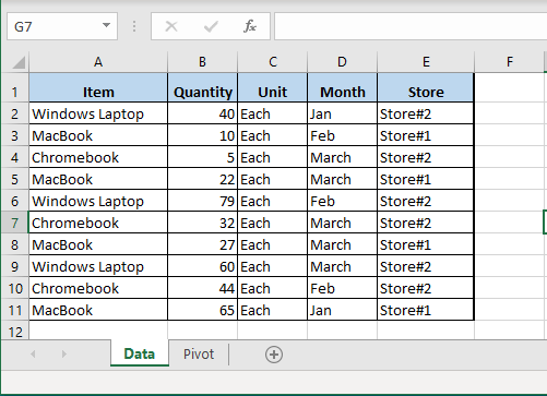
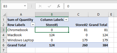
In the example below, we have Sales Data for Windows Laptops, MacBooks and ChromeBooks coming from two different branches of a store.
If the above data is used to create a pivot table with ‘Computers’ in Row Area and ‘Store#1’ in Column Area, we will end up with a Pivot Table having blanks Cells.
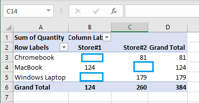
As mentioned above, blank cells in Pivot Table can be seen as missing data, data entry error or calculation mistake.
Replace Blank Cells with Zeros in Excel Pivot Table
You can follow the steps below to replace blank cells with 0 in Excel Pivot Table.
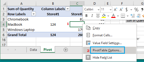
1. Right-click on any Cell within the Pivot Table > select PivotTable Options in the menu that appears.
2. On PivotTable Options screen, select For Empty cells show option and type 0 in the box next to this field.
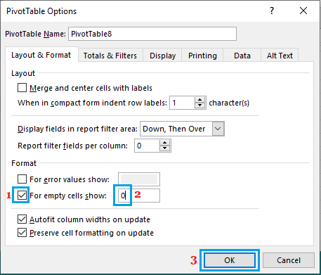
3. Click on OK to save this setting.
4. Once you click on OK, you will immediately see that all the blank cells in the Pivot Table have been replaced with 0.
Note: You can also replace blank cells with any text field (such as “NA” or “No Sales”) by typing NA or No Sales in ‘For Empty Cells Show’ field on Pivot Table Options screen.